Forecasting Returns: What are Reasonable Expectations?
Brighton Jones Investment Committee Update – October 2016
Revisiting Planning Assumptions
As 2015 came to a close, many investors looked ahead to 2016 with a cautious outlook and muted return expectations. Fixed income investors were digesting the Federal Reserve’s first interest rate hike in nearly a decade, while equity investors were battling uneasiness with the fact many broad stock market indices had been trending lower since May. The cautious viewpoints shared by many became firmly entrenched as the US stock market extended its downward trend into early February, culminating in a peak-to-trough decline of about 14%.
Now, with the US bond market (+5.9% YTD) surging and the US stock market (+8.2% YTD) back to recording new highs, the emotional relief of a swift recovery from February’s lows has once again been replaced by concerns about the future. In recent discussions, the two most common questions from our client base have been: (1) what are reasonable forward-looking return expectations, and (2) how do said return expectations factor into the assumptions used in our portfolio sustainability analyses?
In this Investment Committee Update, we will illustrate how investors might derive forward looking return expectations for bonds and stocks, and we then take a deeper dive into the inner workings of Monte Carlo Simulations—the statistical tool we use to measure the long-term sustainability of investment portfolios.
Deriving Expected Bond Returns
Because bonds are contractual obligations that specify the precise timing and amounts of future cash flows (barring default), forecasting the expected return of a bond portfolio is a relatively straightforward exercise.
Assuming an investor maintains a relatively constant mix of bonds (in terms of credit quality and maturities) the most reliable estimate of future returns has historically been the starting yield of the bond portfolio. To demonstrate, we plot historical yields of 10-year Treasuries (x-axis) against subsequent 10-year annualized returns (y-axis):
Visually, we can see that each data point falls very close to the best-fit line (yellow), indicating the predictability of future bond returns is high, although not perfect. This visual observation is supported statistically by the R2 value, which reveals the starting yield of a 10-year Treasury portfolio has historically explained 91% of subsequent returns over 10-year investment periods. It is important to note that predictability is highest when the investment period matches the average maturity of the bonds held. The starting yield of a 30-year bond is not predictive of subsequent returns over a 1-year period, for example, because bond prices do fluctuate in the short-term.
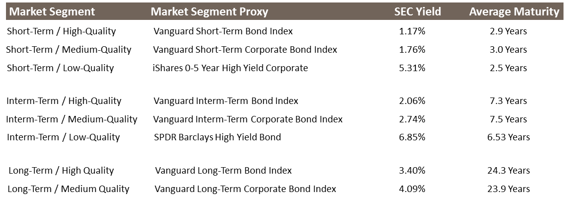
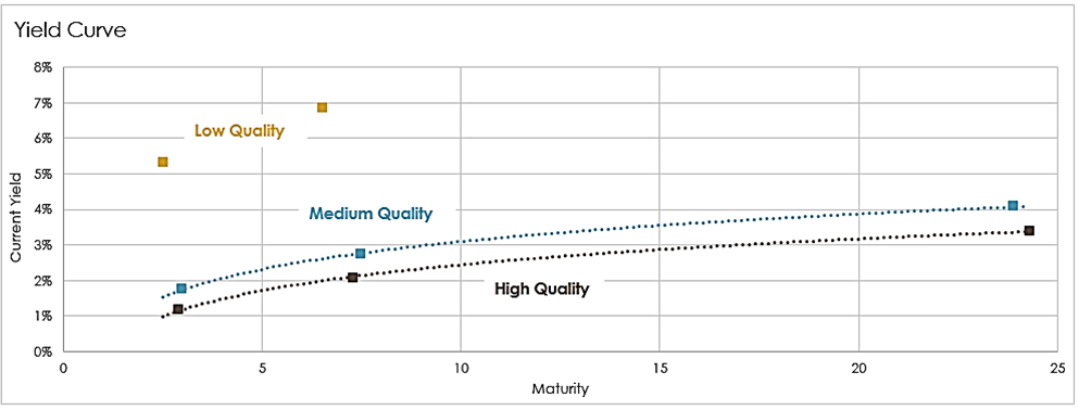
So what might investors expect to earn on fixed income portfolios? In the table below, we list the current yield and average maturity for investment strategies that serve as useful proxies to various bond market segments across the maturity-quality spectrum. As expected, bonds with longer maturities and/or lower credit quality offer higher expected returns. For a bond portfolio diversified across market segments with a bias towards short-to-intermediate maturities and medium-to-high credit ratings, investors may expect to earn about 2.5% over the next decade.
Deriving Expected Equity Returns
Unlike bonds, which are contractual obligations, shareholder equity represents a residual claim (i.e. what’s left over) on assets once all liabilities have been settled. In effect, forecasting the expected return of the stock market is considerably more nuanced because of the uncertain and unspecified timing and amounts of future cash flows.
The most common approach to forecasting future stock market returns is to calculate the market’s Price-to-Earnings Ratio (using the past 12 months of reported earnings) and to compare the prevailing reading to past observations. Conventional wisdom suggests future returns are likely to be above-average when the starting P/E ratio is below-average, and vice versa. Putting this idea to the test, we plot the starting P/E ratio (x-axis) of the S&P 500 Index against subsequent 10-year annualized returns (y-axis):
As expected, there is a downward sloping relationship, suggesting investors would be wise to base intermediate-term planning decisions around below-average returns. More specifically, the best-fit line associates the current P/E reading with about a 6% return over the next decade. Unfortunately, the data does not clearly indicate if and when investors should allocate more or less to equities. There are simply too many examples of relatively cheap markets yielding poor subsequent returns and relatively expensive markets yielding decent subsequent returns to make market timing decisions with a reasonable degree of conviction.
Unsatisfied with such an unreliable indicator, researchers have continued to seek ways to improve the predictive power of the P/E Ratio. In a 1988 paper, economists John Y. Campbell and Robert Shiller made the case for using a 10-year moving average of inflation-adjusted earnings to smooth out short-term earnings volatility and medium-term business cycles in the general economy. We plot the revised approach below, now using the Cyclically-Adjusted P/E Ratio:
The so-called CAPE Ratio offers a clear improvement over the original approach, but once again, there is a very wide range of realized return outcomes for each P/E reading. For example, the best-fit line associates the current P/E reading with an expected 10-year return of about 5 1/2%, but historical observations from periods of comparable market valuation have ranged from slightly negative to as high as 10%.
Over the years, professional investors and academics alike have expended countless resources trying to discover the model that best predicts future stock market returns. But absent a single approach that offers a bond-like degree of predictability, every proposed model is accompanied by pages upon pages of caveats and footnotes.
The one caveat worth addressing here is the relationship between equity market valuations and interest rates. In recent years, many market observers have noted that P/E readings are indeed high (regardless of methodology), but with interest rates so low, investors have nowhere else to go. As such, many have suggested that low interest rates are generally supportive of higher P/E readings. In testing this notion, we plot historical 10-year Treasury yields (x-axis) against CAPE Ratios (y-axis):
On balance, there does appear to be merit to the notion that low interest rates can be supportive of higher valuations, and vice versa. This isn’t to say that investors should expect to continue benefiting from P/E multiple expansion, but the data should at least quell fears that the market is considerably overvalued, as some might suggest. Indeed, equities continue to offer value relative to cash and high-quality fixed income.
So, what should equity investors expect? While stock market forecasts are notoriously unreliable, the various forecasting techniques are in agreement that investors should expect below-average returns over the next decade. The models discussed here place expected returns for the US stock market in the 5-6% range. At the same time, the wide range of realized outcomes during prior periods of comparable market valuation highlights the importance of diversifying growth-oriented investments beyond the domestic stock market. The investable universe includes more than 12,000 companies in 23 developed economies and 23 emerging market economies. History shows that some countries are likely to disappoint while others are likely to surprise, but a globally diversified portfolio is one that mitigates the risk of concentrating assets in the one market segment that delivers disappointing results.
Portfolio Sustainability
As sensibly derived as muted return forecasts might be, the more pressing question is: how does this information factor into the assumptions used in our long-term portfolio sustainability analyses?
By way of background, our portfolio sustainability analyses use a mathematical technique known as the Monte Carlo Method. The technique is used in many fields where practitioners are faced with making decisions under conditions of uncertainty, ambiguity, and variability.
For our purposes, the Monte Carlo Method is an essential tool for optimizing life planning decisions. For those in or approaching retirement, Monte Carlo Simulations help us determine sustainable withdrawal rates for investment portfolios that may need to fund 20-40 years of living expenses. For those in the prime of their career, Monte Carlo Simulations help us set annual savings goals to fund future liabilities, such as retirement, education, second home purchases, and so on.
Of course, the amount of money one client needs to save and another client is able to spend will be largely influenced by the assumed rate of return earned on their respective investment portfolios. If our return assumptions are overly conservative, our clients may have to forego spending as much as they desire now. But, if our return assumptions are overly aggressive, some may be forced to scale back their lifestyle in the future. In effect, basing planning decisions around realistic investment returns is critically important; and the Monte Carlo Method allows us to test different planning scenarios in the presence of return uncertainty and variability.
Revisiting our earlier discussion of expected rates of return, it is important to emphasize that P/E ratios lose predictive power over the long run. For those currently working and saving, structural market factors (i.e. economic growth, population growth, etc.) are likely to prove more important than starting valuations (not to mention the incremental savings of those currently working will be diversified across periods of higher and lower market valuations). On the other hand, our near-term outlook for muted returns has greater potential to impact those currently drawing from their portfolios. Thus, as we proceed with a deeper look at the inner workings and underlying assumptions of our sustainability analyses, we focus our discussion on balanced portfolios currently in drawdown mode.
In our simulations, the assumed average rate of return for a moderately allocated portfolio is 6% and the assumed rate of inflation for general expenses is 3.5%, resulting in an implied inflation-adjusted return of 2.5% (i.e. 6% minus 3.5%). How does the historical data line up with our model inputs?
In the chart below we show rolling 25-year annualized returns of a portfolio allocated 40% to 5-year Treasuries and 60% to US Stocks (grey), less 1.5% to account for frictional costs. Secondly, we show the portfolio returns adjusted for inflation (yellow):
As illustrated, both the stated nominal return of 6% (grey, dotted) and the implied inflation-adjusted return of 2.5% (yellow, dotted) used in our model lie on the lower end of outcomes investors have historically realized over rolling 25-year periods. Thus, for long range planning, the model inputs are relatively conservative.
That said, experiencing adverse market volatility in the first few years of retirement is not only gut-wrenching for recent retirees, but early declines plus ongoing withdrawals can lead to an eventual shortfall in savings. The so-called “sequence-of-returns” risk describes the reality that even if returns average out in the long run, it may not matter if ongoing withdrawals deplete the portfolio before the good returns finally show up. In managing portfolios that may need to fund 20-40 years of lifestyle expenses, it is critically important to account for the “sequence-of-returns” risk, and here’s how we do it:
In deriving sustainable withdrawal rates for those spending down portfolio assets, we can employ one of two methods. We can run a straight-line analysis that assumes a portfolio earns the same rate of return every year, or we can use a Monte Carlo simulator to generate thousands of return series that fall within a specified range (i.e. a probability distribution). We illustrate the difference between the two approaches in the graphic below:
In generating 10,000 sequences of returns, the laws of probability dictate that some series will yield “lucky” results and others will yield “unlucky” results. The “unlucky” series are those with both below-average returns and unfavorable return sequences (i.e. bad returns in the early years of retirement). With thousands of possible outcomes to analyze, the Monte Carlo Method allows us to set near-term spending levels based on one of the more “unlucky” series of returns (i.e. in statistician-speak we are “solving for a high degree of confidence”).
While setting a withdrawal rate based on an “unlucky” series of returns will reduce the amount a retiree is currently able to spend, they will have the option to make adjustments in the future based on what actually happens. If returns turn out to be more favorable than not, spending levels can be increased after a period of time. And in the event returns are less than favorable, they will be less likely to have to make downward adjustments having already planned for a relatively “unlucky” sequence of returns. Now, let’s dive into an example:
In the following illustration, we want to determine the sustainability of spending $42,500 per year inflating at 3.5% per year from a $1,000,000 portfolio over a 25-year time horizon. Based on a moderate allocation, we set up a Monte Carlo simulator to generate 10,000 series of returns with a 6% average and 8% standard deviation.
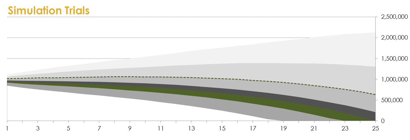
The chart below visually shows the range of simulated outcomes. In some scenarios, we can see the portfolio doesn’t even deplete—it continues to grow; while in other scenarios, we can see the portfolio runs out of money early, failing to reach its 25-year time horizon.
From the results of this simulation, there are three questions worth exploring: (1) can the portfolio really continue to grow, (2) is it actually possible the portfolio will run out of money too soon, and (3) how do we determine if spending $42,500 annually adjusted for inflation is sustainable?
In scenarios where “lucky” outcomes materialize and the portfolio continues to grow, it will become clear that a higher spending level is feasible after a number of years. In such scenarios, it would be up to our client to allow the portfolio to continue growing, or increase the withdrawal rate and begin depleting assets.
Alternatively, other scenarios are clearly “unlucky.” The worst case scenario shows the portfolio running out of money in year 19, failing to reach its 25-year objective. In this scenario, changes would have to be made to extend the longevity of the portfolio. The earlier changes are made, the less drastic they would need to be. For example, simply reducing the rate at which spending inflates each year might be enough to put a plan back on track.
Ultimately, determining the sustainability of a desired spending level is more art than science. Just as it is important not to base spending levels on overly optimistic return assumptions, we also don’t want to unduly constrain the ability of our clients to “live in the now” by basing all planning decisions around worst case scenarios. Our aim, therefore, is to base planning decisions at a level where 75%-80% of our simulations succeed in lasting the full planning period without needing to make future spending cuts.
By setting withdrawal rates based on a 75%-80% confidence level in our simulataions, we are effectively planning around a future that yields below-average returns as well as a relatively unfavorable sequence of returns (i.e. bad returns in the early years of retirement). To illustrate, the table below shows projected outcomes for selected trials from the 10,000 generated in our simulation. We include the outcomes of individual trials ranging from very good (10th percentile) to average (50th percentile) to downright bad (90th percentile):
On the right-hand side of the table, we show the Internal Rates of Return (IRR) for the selected trials over a short-term horizon (5 years) and for the full 25-year period. In focusing on the 75th and 80th percentiles, there are two observations to highlight: (1) the IRRs in year 25 are below the simulation’s stated average return of 6%, and (2) the IRRs through year 5 are lower than those through year 25 (indicating that returns were lower in the earlier years than later on). In effect, “solving for a higher confidence” is equivalent to planning around a below-average rate of return and a less-favorable sequence of returns.
Following a seven-year rally in global equity and fixed income markets, financial securities appear to be priced to offer below-average expected rates of return over the next decade. Indeed, talk about muted returns could prompt a host of actions that, in hindsight, prove to be ill-advised (e.g. stashing cash under a mattress, attempting tactical market timing strategies, chasing the next investment fad to come out of Wall Street, etc.). We reiterate our belief that a balanced, globally diversified portfolio continues to be the best approach to protecting and growing the purchasing power of financial assets, even if the days of double-digit returns are likely behind us for a period of time.
The good news for our clients is that our approach to managing portfolios and planning for the future means that we are prepared for a future that is less favorable than the recent past. By insulating 10-15 years of each client’s anticipated cash needs in a high-quality fixed income portfolio, the portion of assets we hold in growth-oriented investments has ample time to perform. And by setting sustainable withdrawal rates based on relatively unfavorable sequences of returns, our clients are less likely to have to make downward adjustments to their lifestyle in the future.


